Functional Data Engineering

_{written by Maxime Beauchemin}
View original article

Batch data processing — historically known as ETL — is extremely challenging. It’s time-consuming, brittle, and often unrewarding. Not only that, it’s hard to operate, evolve, and troubleshoot.

In this post, we’ll explore how applying the functional programming paradigm to data engineering can bring a lot of clarity to the process. This post distills fragments of wisdom accumulated while working at Yahoo, Facebook, Airbnb and Lyft, with the perspective of well over a decade of data warehousing and data engineering experience.

Let’s start with a quick primer/refresher on what functional programming is about, from the functional programming Wikipedia page:

In computer science, functional programming is a programming paradigm — a style of building the structure and elements of computer programs — that treats computation as the evaluation of mathematical functions and avoids changing-state and mutable data. It is a declarative programming paradigm, which means programming is done with expressions[1] or declarations[2] instead of statements. In functional code, the output value of a function depends only on the arguments that are passed to the function, so calling a function f twice with the same value for an argument x produces the same result f(x)each time; this is in contrast to procedures depending on a local or global state, which may produce different results at different times when called with the same arguments but a different program state. Eliminating side effects, i.e., changes in state that do not depend on the function inputs, can make it much easier to understand and predict the behavior of a program, which is one of the key motivations for the development of functional programming.

Functional programming brings clarity. When functions are “pure” — meaning they do not have side-effects — they can be written, tested, reasoned-about and debugged in isolation, without the need to understand external context or history of events surrounding its execution.

As ETL pipelines grow in complexity, and as data teams grow in numbers, using methodologies that provide clarity isn’t a luxury, it’s a necessity.

Reproducibility

Reproducibility and replicability are foundational to the scientific method. The greater the claim made using analytics, the greater the scrutiny on the process should be. In order to be able to trust the data, the process by which results were obtained should be transparent and reproducible.

While business rules evolve constantly, and while corrections and adjustments to the process are more the rule than the exception, it’s important to insulate compute logic changes from data changes and have control over all of the moving parts.

Let’s take an example where some raw data provided by some other company has been identified as faulty, and the decision has been made to re-import corrected data and reprocess a certain time-range to correct the issue. Now we know that all of the data structures derived from that table, for that time range, need to be reprocessed, or backfilled. In theory, what we want to do is to apply the exact same compute scheme as we did on the original pass, on top of the new, corrected data. Note that it’s also important for the related datasets used in this computation to be identical as they were at the time of the original computation. For example, if one of the downstream processes joins to a dimension to enrich the data, we’d want for that dimension to be identical to how it was when computing the original process. If we cannot provide this guarantee, it implies that performing the same computation, for the same period may yield different results each time it is computed.

Similarly, if we want to change a business rule and perform a backfill all of the downstream computation, we need the guarantee that the change of logic is the only moving part. We need that same guarantee that the blocks of data used in the computation are identical to the ones used when re ran the original process, or in other words, that the sources have have not been altered.

To put it simply, immutable data along with versioned logic are key to reproducibility.

Pure tasks

To make batch processing functional, the first thing is to avoid any form of side-effects outside the scope of the task. A pure task should be deterministic and idempotent, meaning that it will produce the same result every time it runs or re-runs. This requires forcing an overwrite approach, meaning re-executing a pure task with the same input parameters should overwrite any previous output that could have been left out from a previous run of the same task.

Having idempotent tasks is vital for the operability of pipelines. When tasks fail, or when the compute logic needs to be altered for whatever reason, we need the certainty that re-running a task is safe and won’t lead to double-counting or any other form of bad state. Without this assumption, making decisions about what needs to be re-executed requires the full context and understanding of all potential side-effects of previous executions.

Note that contrarily to a pure-function, the pure-task is typically not “returning” an object in the programming sense of the term. In the context of a SQL ELT-type approach which has become common nowadays, it is likely to be simply overwriting a portion of a table (partition). While this may look like a side-effect, you can think of this output as akin to the immutable object that a typical pure-function would return.

Also, for the sake of simplicity and as a best practice, individual tasks should target a single output, the same way that a pure-function shouldn’t return a set of heterogenous objects.

In some cases it may appear difficult to avoid side-effects. One potential solution is to re-think the size of the unit of work. Can the task become pure if it encompasses other related tasks? Can it be purified by breaking down into a set of smaller tasks?

It’s also important that all transitional states within the pure-task are insulated much like locally scoped variables in pure-functions. Multiple instances of the pure task should be fully independent in their execution. If temporary tables or dataframes are used, they should be implemented in a way that task instances cannot interfere with one another so that they can be parallelized.

Table partitions as immutable objects

One of the way to enforce the functional programming paradigm is to use immutable objects. While purely functional languages will prevent mutations by enforcing the use of immutable objects, it’s possible to use functional practices even in a context where the exposed objects are in fact mutable.

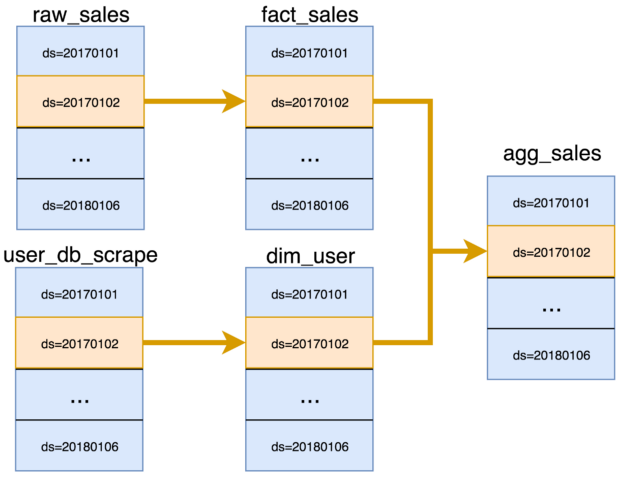
_{a simplified DAG of partitions}

While your database of choice may allow you to update, insert, and delete at will, it doesn’t mean you should. DML operations like UPDATE, APPEND and DELETE are performing mutations that ripple in side-effects. Thinking of partitions as immutable blocks of data and systematically overwriting partitions is the way to make your tasks functional. A pure task should always fully overwrite a partition as its output.

Your data store may not have support for physical partitions, but that does not prevent you from taking a functional approach. To work around this limitation, one option is to implement your own partitioning scheme by using different physical tables as the output of your pure tasks that can be UNIONed ALL into views that act as logical tables. Results may vary depending on how smart your database optimizer is. Alternatively, it’s also possible to logically partition a table and to systematically DELETE prior to INSERTing using a partitioning key that reflects the parameters used to instantiate the task. Note that where a TRUNCATE PARTITION is typically a “free” metadata operation, a DELETE operation may be expensive and that should be taken into considerations. If you decide to go that route, note that on many database engines it may more efficient to check whether the DELETE operation is needed first to avoid unnecessary locking.

A persistent and immutable staging area

The staging area is the conceptual loading dock of your data warehouse, and while in the case a real physical retail-type warehouse you’d want to use a transient staging area and keep it unobstructed, in most modern data warehouse you’ll want to accumulate and persist all of your source data there, and keep it unchanged forever.

Given a persistent immutable staging area and pure tasks, in theory it’s possible to recompute the state of the entire warehouse from scratch (not that you should), and get to the exact same state. Knowing this, the retention policy on derived tables can be shorter, knowing that it’s possible to backfill historical data at will.

Changing logic over time

Business logic and related computations tend to change over time, sometimes in retroactive fashion, sometimes not. When retroactive, you can think of the change as making existing downstream partitions “dirty” and it calls for them to be recomputed. When non-retroactive, the ETL logic should capture the change and apply the proper logic to the corresponding time range. Logic that changes over time should always be captured inside the task logic and be applied conditionally when instantiated. This means that ideally the logic in source control describes how to build the full state of the data warehouse throughout all time periods.

For example, if a change is introduced as a new rule around how to calculate taxes for 2018 that shouldn’t be applied prior to 2018, it would be dangerous to simply update the task to reflect this new logic moving forward. If someone else was to introduce an unrelated change that required “backfilling” 2017, they would apply the 2018 rule to 2017 data without knowing. The solution here is to apply conditional logic within the task with a certain effective date, and depending on the slice of data getting computed, the extra tax logic would apply where needed.

Also note that in many cases business rules changes over time are best expressed with data as opposed to code. In those cases it’s desirable to store this information in “parameter tables” using effective dates, and have logic that joins and apply the right parameters for the facts being processed. An oversimplified example of this would be a “taxation rate” table that would detail the rates and effective periods, as opposed to hard-coded rates wrapped in conditional blocks of code.

But what about dimensions?

By nature, dimensions and other referential data is slowly changing, and it’s tempting to model this with UPSERTs (UPdating what has changed and inSERTing new dimension members) or to apply other slowly-changing-dimension methodology to reflect changes while keeping track of history. But how do we model this in a functional data warehouse without mutating data?

Simple. With dimension snapshots where a new partition is appended at each ETL schedule. The dimension table becomes a collection of dimension snapshots where each partition contains the full dimension as-of a point in time. “But only a small percentage of the data changes every day, that’s a lot of data duplication!”. That’s right, though typically dimension tables are negligible in size in proportion to facts. It’s also an elegant way to solve SCD-type problematic by its simplicity and reproducibility. Now that storage and compute are dirt cheap compared to engineering time, snapshoting dimensions make sense in most cases.

While the traditional type-2 slowly changing dimension approach is conceptually sound and may be more computationally efficient overall, it’s cumbersome to manage. The processes around this approach, like managing surrogate keys on dimensions and performing surrogate key lookup when loading facts, are error-prone, full of mutations and hardly reproducible.

In case of very large dimensions, mixing the snapshot approach along with SCD-type methodology may be reasonable or necessary. Though in general it’s sufficient to have the current attribute only in the current snapshot, and denormalize dimension attributes into fact table where the attribute-at-the-time-of-the-event is important. For the rare cases where attribute-at-the-time-of-the-event importance was not foreseen and denormalized into fact upfront, you can always run a more expensive query that joins the facts to their time-relative dimension snapshots as opposed to the latest snapshot.

You could almost think about the “dimension snapshotting” approach as a type of further denormalization that has similar tradeoffs as other types of denormalization.

Another modern approach to store historical values in dimensions is to use complex or nested data types. For example if we wanted to keep track of the customer’s state over time for tax purposes, we could introduce a “state_history” column as a map where keys are effective dates and values are the state. This allows for history tracking without altering the grain of the table like a type-2 SCD requires, and is much more dynamic than a type-3 SCD since it doesn’t require creating a new column for every pice of information.

Unit of work

Clarity around the unit of work is also important, and the unit of work should be directly aligned to output to a single partition. This makes it trivial to map each logical table to a task, and each partition to a task instance. By being strict in this area it makes it easy to directly map each partitions in your data store to its corresponding compute logic.

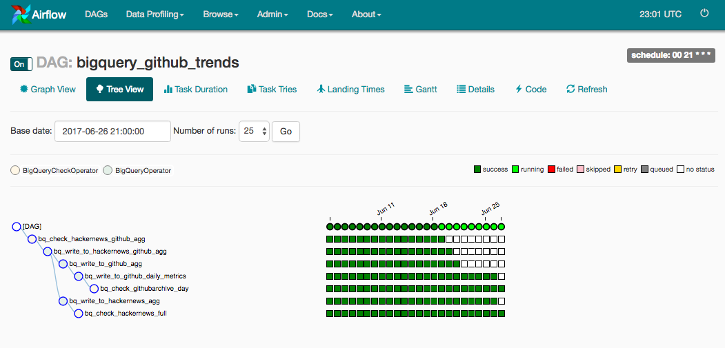
For example, in this Airflow “tree view” where squares represents task instances of a DAG of tasks over time, it’s comforting to know that each row represents a task that corresponds to a table, and that each cell is a task instance that corresponds to a partition. It’s easy to track down the log file that correspond to any given partition. Given that tasks are idempotent, re-running any of these cells is a safe operation. This set of rule makes everything easier to maintain since a clear scope on the units of work make everything clear and maintainable.

As a side note, Airflow was designed with functional data engineering in mind, and provides a solid framework to orchestrate idempotent, pure-tasks at scale. Full disclosure is due here, the author of this post happens to be the creator of Airflow, so no wonder the tooling works well with the methodology prescribed here.

A DAG of partitions

While you may think of your workflow as a directed acyclic graph (DAG) of tasks, and of your data lineage as a graph made of tables as nodes, the functional approach allows you to conceptualize a more accurate picture made out of task instances and partitions. In this more detailed graph, we move away from individual rows or cells being the “atomic state” that can be mutated to a place where partitions are the smallest unit that can be changed by tasks.

This data lineage graph of partitions is much easier to conceptualize to the alternative where any row could have been computed by any task. With this partition-lineage graph, things become clearer. The lineage of any given row can be mapped to a specific task instance through its partition, and by following the graph upstream it’s possible to understand the full lineage as a set of partitions and related task instances.

Past dependencies

A common pattern that leads to increased “state complexity” is when a partition depends on a previous partition on the same table. This leads to growing complexity linearly over time. If for instance, computing the latest partition of your user dimension uses the previous partition of that same table, and the table has 3 years of history with daily snapshot, the depth of the resulting graph grows beyond a thousand and the complexity of the graph grows linearly over time. Strictly speaking, if we had to reprocess data from a few months back, we may need to reprocess hundreds of partition using a DAG that cannot be parallelized.

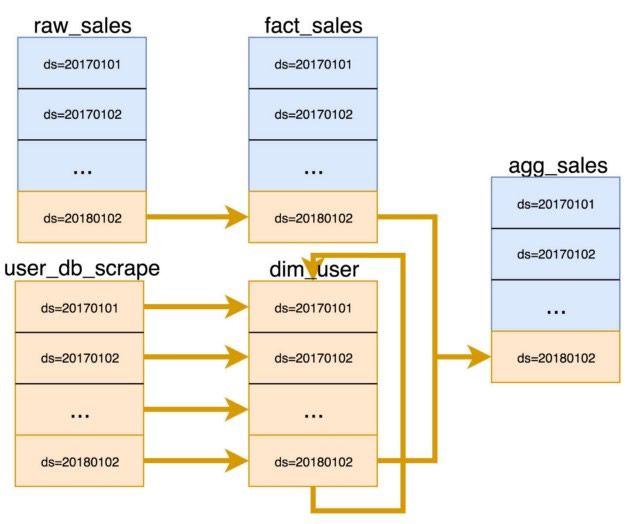
_{simplified DAG of partitions with a past dependency}

Given that backfills are common and that past dependencies lead to high-depth DAGs with limited parallelization, it’s a good practice to avoid modeling using past-dependencies whenever possible.

In cases where cumulative-type metrics are necessary (think live-to-date customer spending as part of a customer dimension for instance), one option is to model the computation of this metric in a specialized framework or somewhat independent model optimized for that purpose. A cumulative computation framework could be a topic for an entire other blog post, let’s leave this out of scope for this post.

Late arriving facts

Late arriving facts can be problematic with a strict immutable data policy. Unfortunately late arriving data is fairly common, especially in given the popularity of mobile phones and occasional instability of networks.

To bring clarity around this not-so-special case, the first thing to do is to dissociate the event’s time from the event’s reception or processing time. Where late arriving facts may exist and need to be handled, time partitioning should always be done on event processing time. This allows for landing immutable blocks of data without delays, in a predictable fashion.

This effectively brings in two tightly related time dimensions to your analytics and allows to do intricate analysis specific to late-arriving facts. Knowing when events were reported in relation to when they occurred is useful. It allows for showing figures like “total sales in February as of today”, “total sales in February as of March 1st” or “how much sales adjustments on February since March 1st”. This effectively provides a time machine that allows you to understand what reality looked like at any point in time.

When defining your partitioning scheme based on event-processing time, it means that your data is not longer partitioned on event time, and means that your queries that will typically have predicates on event time won’t be able to benefit from partition pruning (where the database only bothers to read a subset of the partitions). It’s clearly an expensive tradeoff. There are a few ways to mitigate this. One option is to partition on both time dimensions, this should lead to a relatively low factor of partition multiplication, but raises the complexity of the model. Another option is to author queries that apply predicates on both event time and on a relatively wider window on processing time where partition pruning is needed. Also note that in some cases, read-optimized stores may not suffer much from the inability the database optimizer to skip partitions through pruning as execution engine optimizations can kick in to reach comparable performance. For example, if your engine is processing ORC or Parquet files, the execution will be limited to reading the file header before moving on to the next file.

A standard deviation

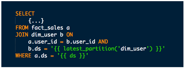
Rules are meant to be broken and in some cases it’s rational to do so. A common pattern we’ve observed is to trade perfect immutability guarantees in exchange for earlier SLAs (Service License Agreement on acceptable delays make data available). Let’s take an example where we want to compute aggregates that depend on the user dimension, but that this user dimension usually lands very late in the day. Perhaps we care more about our aggregate landing early in the day than we care about accuracy. Given this preference, it’s possible to join onto the latest partition available at the time the other dependencies are met. Note that this can easily limited to a specified time range (say 2–3 partitions) to insure a minimum level of accuracy. Of course this means that re-processing the aggregation table later in the future may lead to slightly different results.

In retrospect

While this post may be a first in formalizing the functional approach to data engineering, these practices aren’t experimental or new by any means. Large, data driven, analytically mature corporations have been applying these methods for years, and reputable tooling that prescribes this approach has been widely adopted in the industry.

It’s clear that the functional approach contrasts with with decades of data-warehousing literature and practices. It’s arguable that this new approach is more aligned with how modern read-optimized databases function as they tend to use immutable blocks or segments and typically don’t allow for row-level mutations. This methodology also skews on treating storage as cheap and engineering time as expensive, duplicating data for the sake of clarity and reproducibility.

At the time where Ralph Kimball authored The Data Warehouse Toolkit, databases used for warehousing were highly mutable, and data teams were small and highly specialized. Things have changed quite a bit since then. Data is larger, read-optimized stores are typically built on top of immutable blocks, we’ve seen the rise of distributed systems, and the number and proportion of people partaking in the “analytics process” has exploded.

More importantly, given that this methodology leads to more manageable and maintainable workloads, it empowers larger teams to push the boundaries of what’s possible further by using reproducible and scalable practices.

View original article

_{*Source: Medium}